Each element of any computer model comes with uncertainty – imprecision springing from indefinite data, poorly understood physical properties and inexactness in the model’s recreation of reality. The big question: How can scientists calculate the degree of possible error in their models? Exploring that question lies at the heart of uncertainty quantification, known to the experts simply as UQ.
Because UQ requires large computing capabilities, calculating error in many scientific computations today remains more theory than practice, says Habib Najm, a distinguished member of the technical staff at Sandia National Laboratories’ Livermore, Calif., site.
The advent of exaflops-capable computers – roughly a thousand times faster than today’s supercomputers – later this decade may provide the extra power needed for UQ on today’s simulations. UQ also will be important in understanding how much confidence to place in the highly detailed models exascale computing will enable.
For that reason, UQ is a major part of the Department of Energy Advanced Scientific Computing Research office’s exascale-computing portfolio, which includes a project Najm leads called QUEST, for Quantification of Uncertainty in Extreme Scale Computations. Sandia’s QUEST collaborators are Los Alamos National Laboratory, Johns Hopkins University, Massachusetts Institute of Technology and the universities of Southern California and Texas at Austin.
‘If you know something about the behavior of a system, you can take advantage of that knowledge and reduce the number of sample points.’
Uncertainty often is described as a distribution of values within which a particular observed value could fall. To quantify it in predictions from a simulation, scientists start by identifying sources of uncertainty in parameters that make up the model – the variables that affect the output. Next, they typically perform sensitivity analysis, identifying the parameters whose uncertainty affects predictions the most. This uncertainty then can be propagated through a model to reveal how it changes a simulation’s output.
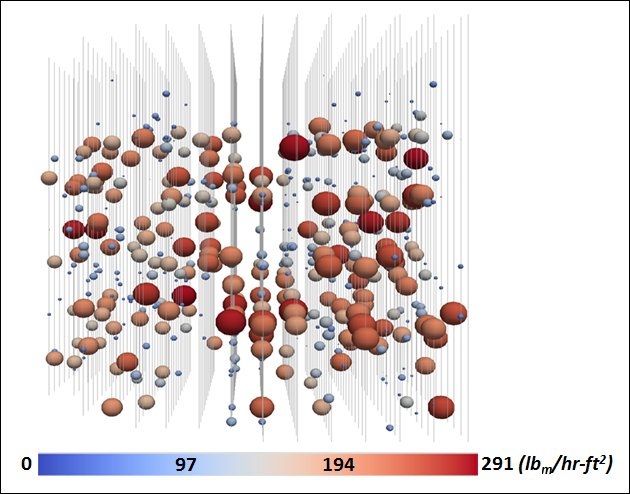
Uncertainty analysis can also help scientists understand the processes inside a nuclear reactor core, as shown here. This side view of a quarter core includes vertical lines that indicate fluid-flow channels and the spheres portray localized boiling. The color of the spheres indicates the boiling rate – lower for blue and higher for red – and the size of a sphere indicates its uncertainty. Image courtesy of Michael S. Eldred, Sandia National Laboratories.
Michael S. Eldred, distinguished member of the technical staff at Sandia’s Albuquerque, N.M., site, offers context for that last step: “The goal of uncertainty propagation, put simply, is to take distributions on the things that you know and propagate them to what you don’t know.” For example, a researcher could estimate the uncertainty in a thermal boundary condition and use it to compute uncertainty in temperature predictions at a crucial region in the modeled system.
To perform this type of propagation, a researcher typically runs the simulation many times using varied inputs – enlisting, for example, Monte Carlo sampling methods that select inputs randomly from a set of possibilities, then statistically analyzes the ensemble of outputs.
Researchers also employ more efficient techniques, such as polynomial chaos methods, to propagate uncertainty. Dongbin Xiu, associate professor of mathematics at Purdue University, explored this approach in Numerical Methods for Stochastic Computations: A Spectral Method Approach (Princeton University Press 2010).
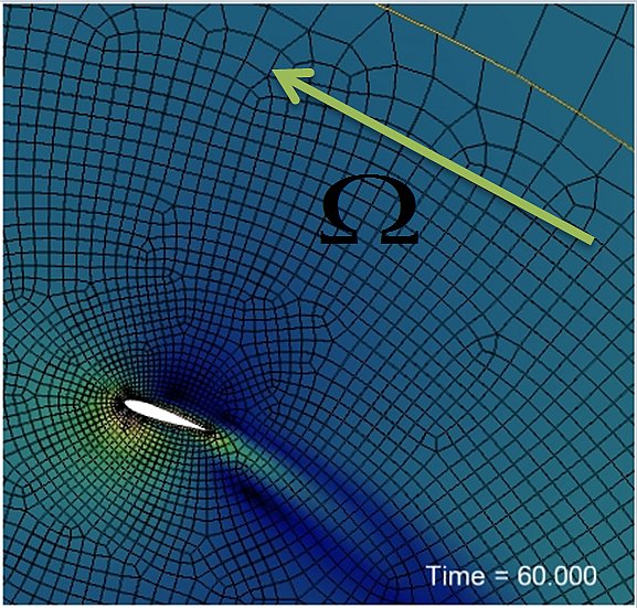
Uncertainty analysis can be applied to a wide range of simulations, including this ASCR project that modeled wind turbines. Image courtesy of Michael S. Eldred, Sandia National Laboratories.
Xiu describes this technique as a “Fourier method in random space.” That allows it to model uncertain variables as random and reach a solution “very fast and with decent accuracy at a much reduced computational effort.”
UQ experts face a range of obstacles when seeking uncertainty sources. A key challenge, Najm says, is “the high dimensionality of models” – the large number of uncertain parameters that complicate computing the variability in a simulation’s output.
 Nonlinearity adds other twists. “When models are nonlinear,” Najm says, “they tend to amplify any uncertainties that go into them.” Consequently, a small change in an input can spawn a large, unexpected change in the output.
The elements that comprise a simulation also contribute to uncertainty. For example, a model’s geometry will not exactly reproduce the geometry of the real-world system. Equations used to model the real-world physics also supply uncertainty.
Another factor contributing to uncertainty: each variable’s initial conditions. Models often rely on parameters that were estimated from sources that range from empirical data to other calculations. “You rarely have the luxury of having the data to characterize uncertainty as you would like,” Najm says.
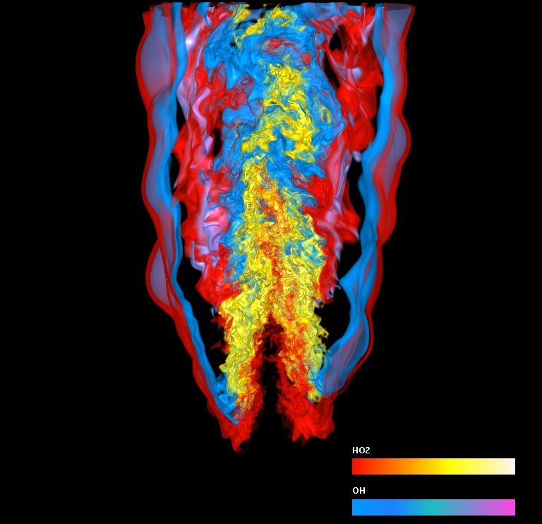
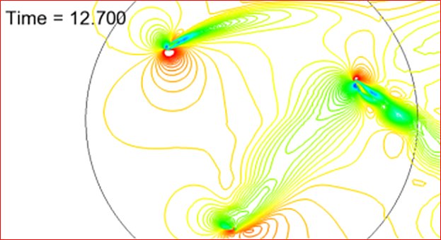
Simultaneous visualization of two variables of a turbulent combustion simulation performed by Jacqueline Chen, Sandia National Laboratories. Credit: Hongfeng Yu, University of California at Davis.
Najm and his colleagues use UQ on a range of thermo-fluid problems, including combustion. Simulating burning of even a simple hydrocarbon like methane in air requires about 300 reactions, each based on about three parameters – meaning a simulation involves about 1,000 uncertain parameters. As Najm says, “For more complex fuels, we’re starting to talk about 3,000 reactions and up to 10,000 reactions. The number of uncertain parameters grows very quickly.”
To make UQ in combustion even more daunting, a parameter’s uncertainty might spread over a factor of 10 up or down.
Sensitivity analysis can reduce the number of parameters that must be considered. “You may have large uncertainties in some parameters, but it may not matter,” Najm says. Conversely, a parameter with smaller uncertainty might have far more impact on the output.
Working on nuclear-stockpile stewardship through Lawrence Livermore National Laboratory’s Advanced Simulation and Computing Program, Charles Tong, a member of the lab’s technical staff, developed a UQ software library called PSUADE (Problem Solving environment for Uncertainty Analysis and Design Exploration). “It’s a library of non-intrusive UQ methods, which means that the application code does not have to be modified for each simulation,” Tong says.
Non-intrusive methods rely on sampling and analysis. To limit the required run time, the method depends on finding ways to sample in the most sensitive ranges – say, particular values of specific parameters that play the largest roles in the overall model’s uncertainty – and powerful methods of analyzing the results.
As Tong says, “If you know something about the behavior of a system, you can take advantage of that knowledge and reduce the number of sample points.”
It also might be possible to combine non-intrusive methods with intrusive ones. Tong is researching such hybrid approaches. “Given a complex system, the idea is to break it into components and use the most appropriate uncertainty propagation methods – intrusive or non-intrusive – for each component and then put them together to propagate uncertainties globally.”
Beyond stockpile stewardship, Tong also is applying his UQ software to environmental management applications.
In some cases, a simulation’s complexity makes it difficult to know where to start. Imagine a long time-scale global climate simulation with 5,000 random inputs. It takes a month to run on a big computer and a researcher wants to simulate the likelihood that a rare effect occurs far out in the tails of an output distribution. That’s a worst-case scenario, says Sandia’s Eldred, because it requires a very large number of simulations when only a few are affordable.
To deal with such problems, UQ researchers seek smart adaptive methods, which Eldred says can do more with less. Simply put, such an approach would figure out where it is most important to explore variation and focus simulations in those spots.
Eldred says today’s adaptive methods usually can figure out the subset of the most important parameters without relying on screening derived from theory. “If the important subset is still very large, then we may be highly constrained in what we can do,” he says, although many simulations have far fewer important elements.
Today’s adaptive methods face several challenges. One, Eldred says, is non-smoothness –a “relationship with respect to a set of random variables (in which) the response is discontinuous, noisy or otherwise poorly behaved. The machinery that we’d like to use has to address these difficulties.”
It’s still complicated to develop an adaptive approach that works quickly for a broad range of problems. Eldred and his colleagues have been developing DAKOTA, a UQ toolkit he says “gets the tools in the hands of users and helps remove some of the barriers to performing UQ.”
To further expand UQ’s application, researchers should put more time in capacity-based methods, Purdue’s Xiu says. That is, given a specific amount of computing resources, what is the optimum UQ method?
As Xiu says, “The best that I can achieve with the given resource might not be superb, but it is the best I can do under the constraint. And something is better than nothing.”